IEEE GRSS Hyperspectral Data

Hi everyone. Outside of software development, we also do some work in geoscience and remote sensing. As a result, we were very excited to see an announcement from the IEEE GRSS that they were making some new data sets available - in particular, a hyperspectral data set, and a LIDAR data set (if you’re not familiar with these technologies, see here: http://en.wikipedia.org/wiki/Hyperspectral_imaging and http://en.wikipedia.org/wiki/LIDAR).

Getting Started
A Note About UnLabeled Points
Visualization of the Hyperspectral and LIDAR data
Hyperspectral Data
PC Projections
15-Class Classification
Evaluation
Conclusions

Getting Started

We’ve made some M-files that will load in the data for you (see the .ZIP file at the end of this post), but you’ll need to go to the GRSS website to download the data from here first: http://hyperspectral.ee.uh.edu/?page_id=459).

To load the data, first download the .ZIP file at the end of this post, then run the following. But change the line below to point to the right directory, so for example, I have a file C:\Users\pete\Documents\data\2013IEEE_GRSS_DF_Contest\2013_IEEE_GRSS_DF_Contest_CASI.tif

imgSize = [349 1905];
grssDir = 'C:\Users\pete\Documents\data\2013IEEE_GRSS_DF_Contest\';
[dsCasi,dsLidar] = prtExampleReadGrss2013(grssDir);

Note, if you don’t want to use the PRT for anything, but would like to automatically read in the ROI file provided by GRSS, download the .ZIP at the end of this file, and just use:

regions = grssRoiRead(roiFile);

Each of these data sets has 664845 observations (from the 349x1905 dimensional image) the hyperspectral data has 144 dimensions, and the LIDAR data only has one dimension. The fine folks at GRSS were kind enough to provide labels for about 2832 pixels from the data sets. These are from 15 different classes: grass_healthy, grass_stressed, grass_synthetic, tree, soil, water, residential, commercial, road, highway, railway, parking_lot1, parking_lot2, tennis_court, running_track.

A Note About UnLabeled Points

This data set contains a lot of unlabeled data. Previously, to use the PRT with unlabeled data required ad-hoc fiddling with targets and classes. But as of Jan 7, 2013, the PRT now handles unlabeled data inherently. The PRT uses NaNs to represent unlabeled data points - e.g.,

numNan = length(find(isnan(dsCasi.targets))); %there are 662013 unlabeled points
disp(numNan)

You can get a data set using only the labeled data using new mthods included specifically for unlabeled data:

dsUnLabeled = dsCasi.removeLabeled;
dsLabeled = dsCasi.retainLabeled;

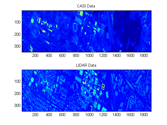
Visualization of the Hyperspectral and LIDAR data

We can visualize the data in the form of the spatial image by re-sizing it to be the correct dimensionality. For example, the next lines reshape the total intensity (SUM) of the hyperspectral data, and reshape the LIDAR data into the right size:

x = dsCasi.X;
x = reshape(x',[144 imgSize]);
imgCasi = sqrt(squeeze(sum(x.^2)));

subplot(2,1,1);
imagesc(imgCasi)
title('CASI Data');

xLidar = dsLidar.X;
imgLidar = reshape(xLidar,imgSize);
subplot(2,1,2);
imagesc(imgLidar)
title('LIDAR Data');

Hyperspectral Data

The remainder of this blog entry will just show a few examples of how to use the PRT in combination with the CASI hyperspectral data; I want to be clear that we’re not doing anything that’s particularly well-motivated from a hyperspectral data perspective. If you’re interested, there’s a great deal of research in the hyperspectral field – we can’t summarize all the interesting stuff that’s going on there, but if you’re interested, check out some recent issues of WHISPERS: http://www.ieee-whispers.com/

In reality, the purpose of the data set from GRSS is to do data fusion, but for today we’ll just be concerned with the hyperspectral data – dsCasi.

PC Projections

As an example, we can explore the data in principal component space. It’s easy enought to do – we can treat the CASI part of the data just like any other prtDataSet. Let’s build an algorithm to do some standard pre-processing. Each 144 dimensional hyperspectral vector is a row of the data matrix, so we can zero-mean, and normalize the standard deviation of each row with prtPreProcZeroMeanRows and prtPreProcStdNormalizeRows (which is new).

preProc = prtPreProcZeroMeanRows + prtPreProcStdNormalizeRows(‘varianceOffset’,10) + prtPreProcPca(‘nComponents’,3);

dsLabeled = dsCasi.retainLabeled;
preProc = preProc.train(dsLabeled);
dsPreProc = preProc.run(dsLabeled);
subplot(1,1,1);
plot(dsPreProc);
legend(‘location’,‘EastOutside’)
title(‘CASI Hyperspectral PC’);

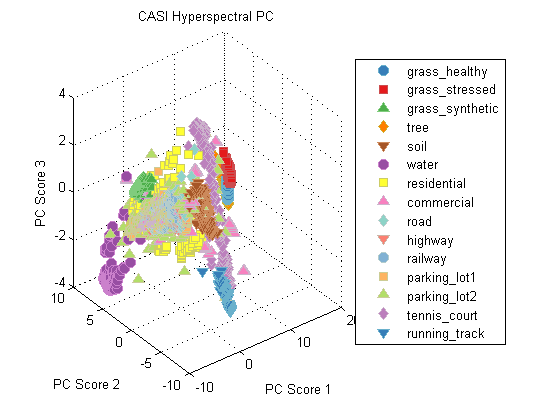
Visualizing the data in PC space, we can see a few things. First, all of the grass and tree samples are quite similar in PC space. Also, synthetic grass looks nothing like the real grass classes – from a hyperspectral perspective, synthetic grass is clearly a man-made material, despite the color similarity between it and real grass.

15-Class Classification

Let’s take a look at doing some classification. Recall that GRSS labeled 15 unique classes for us; we can do standard machine learning with that data. We will use similar pre-processing as above, and then a 15 component PLSDA classifier. PLSDA is nice in this case, since it natively handles multi-class problems, and its quite fast. We can probably get better results with a non-linear classifier, but for now we’ll stick with PLSDA.

dsLabeled = dsCasi.retainLabeled;

algo = prtPreProcZeroMeanRows + prtPreProcStdNormalizeRows(‘varianceOffset’,10) + prtClassPlsda(‘nComponents’,15) + prtDecisionMap;
yOut = algo.kfolds(dsLabeled,3);

close all;
prtScoreConfusionMatrix(yOut);
pc = prtScorePercentCorrect(yOut);
title(sprintf(‘15 Class Classification; %.2f%% Correct’,pc*100));
xlabel(‘’);
rotateticklabel(gca,45);

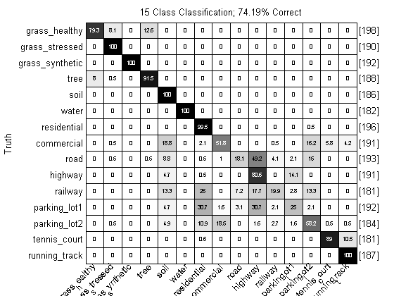
Over 70% correct, with just this simple processing! That’s not too shabby. Note, however, that the cross-validation approach we’ve used here is a little suspect – a lot of the truth proivded to us was from neighboring pixels. These pixels might be only about a meter apart, and two hyperspectral vectors from that close proximity, on, say, grass, will be expected to be much more correlated than two pixels from hundreds of meters apart.

One way to overcome this would be to build cross-validation folds using the spatial locations of the pixels; it would be interesting to see how cross-validation would work under that case.

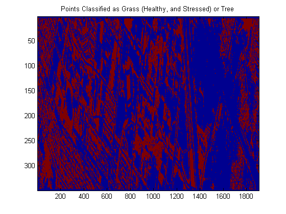
Evaluation

To evaluate our algorithm we can visualize the performance on the entire larger hyperspectral image. First, we run the algorithm, then get the estimated labels, and reshape to the right size for visualization.

algo = algo.train(dsLabeled);
yOutFull = algo.run(dsCasi);

close all;
img = reshape(yOutFull.X,imgSize);
imagesc(img);
colorbar
% It’s a little hard to judge, but this doesn’t look completely
% unreasonable….
%
% The following shows only the points labeled as one of the two types of
% grasses or trees
imagesc(img == 1 | img == 2 | img == 4);
title(‘Points Classified as Grass (Healthy, and Stressed) or Tree’);

Conclusions

If you’re interested in hyperspectral data, LIDAR, or data fusion, you should definitely check out the GRSS data set. We hope the PRT files we’re providing will help you get started.

There’s a lot more to do with this data – we haven’t even explored the LIDAR data yet, or how to fuse information from the two. This data is also a prime candidate for semi-supervised learning (http://en.wikipedia.org/wiki/Semi-supervised_learning), active learning (http://en.wikipedia.org/wiki/Active_learning), or multi-task learning (http://en.wikipedia.org/wiki/Multi-task_learning).

Hopefully we’ll get a chance to delve more into this data set in the near future. Let us know if you have any luck with this data!

Here’s a link to the .ZIP file with all the code you’ll need.

You may also need rotateticklabel.m, which is available from MATLAB Central

PRT Blog