Hi! Today I’d like to talk about how you can use the PRT to combine actions together to form algorithms. This is an important and powerful tool in the PRT, and understanding it can solve a lot of headaches for you.

Contents

An Example

Let’s start with a concrete example. Say we want to classify some very high dimensional data. We’ll start with the following:

nFeatures = 200;
ds = prtDataGenUnimodal;
xNoise = randn(ds.nObservations,nFeatures);
ds.X = cat(2,ds.X,xNoise); %add nFeatures meaningless features

If we try and classify this with a GLRT, for example, we’re going to run into trouble, since there are more features than there are observations, so we can’t generate a full-rank covariance structure. For example, using the prtAction prtClassGlrt, we might write this:

glrt = prtClassGlrt;
glrt = glrt.train(ds);
try
   yOut = glrt.run(ds);  %This causes errors
catch ME
    disp('Error encountered:')
    disp(ME);
end

Warning: Covariance matrix is not positive definite. This may cause errors.
Consider modifying "covarianceStructure". 
Warning: Covariance matrix is not positive definite. This may cause errors.
Consider modifying "covarianceStructure". 
Error encountered:
  MException
  Properties:
    identifier: 'prtRvUtilMvnLogPdf:BadCovariance'
       message: 'SIGMA must be symmetric and positive definite.'
         cause: {0x1 cell}
         stack: [9x1 struct]

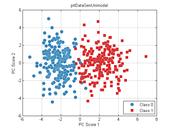
We can always use dimension-reduction techniques to reduce the number of features in our data set, and then evaluate performance. For example:

pca = prtPreProcPca('nComponents',2);
pca = pca.train(ds);
dsPca = pca.run(ds);
plot(dsPca);

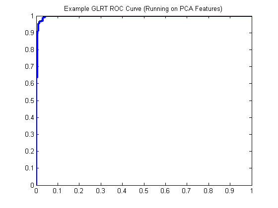
Now we can evaluate our GLRT on the dsPca:

glrt = prtClassGlrt;
yOutKfolds = glrt.kfolds(dsPca,10);
[pf,pd] = prtScoreRoc(yOutKfolds);
h = plot(pf,pd);
set(h,‘linewidth’,3);
title(‘Example GLRT ROC Curve (Running on PCA Features)’);

The Problem

There’s a problem in the above, though. Even though we cross-validated the GLRT using 3 random folds, we didn’t do the same thing with the PCA. This is technically not fair, since the PCA part of the algorithm was trained using all the data.

Maybe we can get around this like so:

pca = prtPreProcPca(‘nComponents’,2);
dsPca = pca.kfolds(ds,10);

But now, when we do:

glrt = prtClassGlrt;
yOutKfolds = glrt.kfolds(dsPca,10);
[pf,pd] = prtScoreRoc(yOutKfolds);
h = plot(pf,pd);
set(h,‘linewidth’,3);
title(‘This is no good…’);

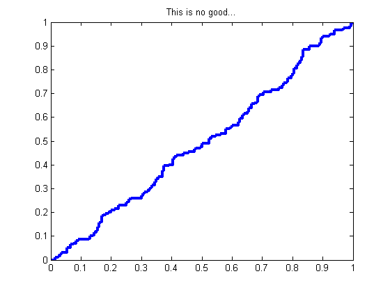
We have a problem! At every fold, we learn a unique set of PCA loadings. Since PCA loadings have arbitrary sign (+/–), the outputs across all these folds will overlap!

plot(dsPca)

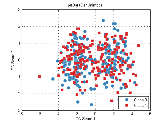
The underlying problem is that there’s no guarantee that the folds used for PCA and GLRT evaluation were the same. We can get around that if we specified the folds, and wrote our own cross-validate specifically for this new process we’ve made, but suddenly this is getting complicated.

And what if we had an even more complicated process, including other pre-processing streams, feature selection, classifiers and decision-makers? Suddenly our code is going to be a mess!

Combining Actions into Algorithms

At the heart of the problem outlined above is that the PCA and GLRT parts of our process weren’t considered as two parts of the same process – they were two separate variables, and the PRT and MATLAB didn’t know that they should work together.

Since this problem is so common, the PRT provides an easy way to combine each individual part of a process (prtActions) into one big process (a prtAlgorithm). This is easily done using the “+” operator:

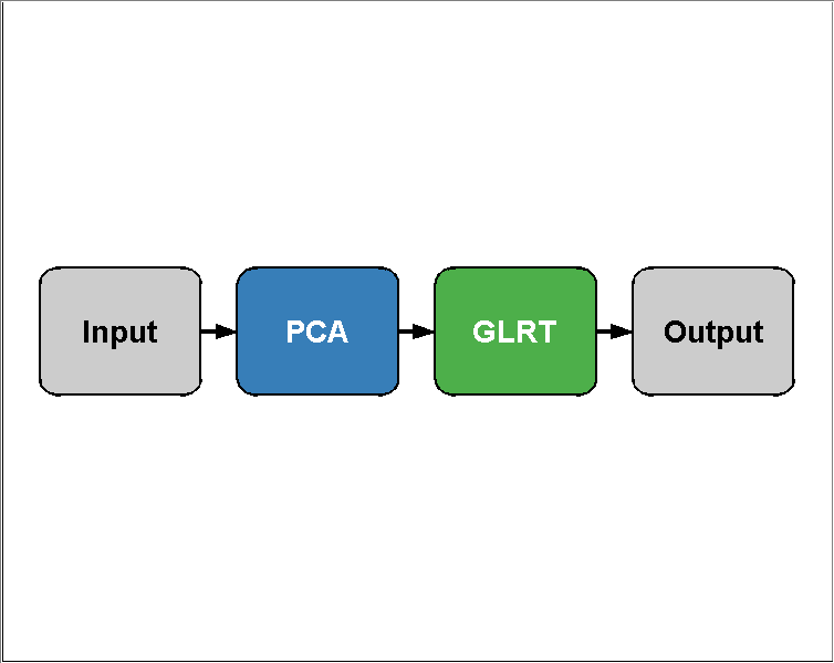
pcaGlrt = prtPreProcPca(‘nComponents’,2) + prtClassGlrt;

If you’re not used to object oriented programming, the above might look a little weird. But it’s straightforward – we’ve defined “plus” (“+”) for prtActions (e.g., prtPreProcPca) to mean “Combine these into one object, where that object will perform each action in sequence from left to right”. Technically this returns a special kind of prtAction, called a prtAlgorithm. That’s just the date type we use to store a bunch of actions. You can see that here:

disp(pcaGlrt)

  prtAlgorithm


  Properties:

                name: 'PRT Algorithm'
    nameAbbreviation: 'ALGO'
        isSupervised: 1
isCrossValidateValid: 1
          actionCell: {2x1 cell}
  connectivityMatrix: [4x4 logical]
      verboseStorage: 1
     showProgressBar: 1
           isTrained: 0
      dataSetSummary: []
             dataSet: []
            userData: [1x1 struct]

You can visualize the structure of the algorithm using PLOT:

plot(pcaGlrt)

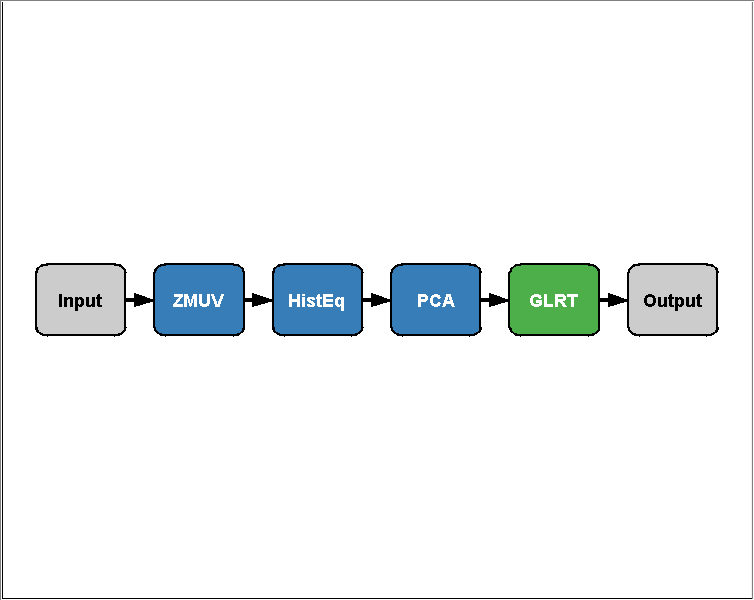
You can combine any number of prtActions into an algorithm like this, so, although its silly, this is technically a valid command:

sillyAlgo = prtPreProcZmuv + prtPreProcHistEq + prtPreProcPca + prtClassGlrt;
plot(sillyAlgo)

Using Algorithms

So we’ve made a prtAlgorithm. Now what? Well, anything you can do to a prtAction, you can do with a prtAlgorithm. What does that mean? Methods like plot, kfolds, and crossValidate all work exactly the same as they do with regular prtActions. And they make your life much simpler than what we had to do above:

pcaGlrt = prtPreProcPca(‘nComponents’,2) + prtClassGlrt;
yOutKfolds = pcaGlrt.kfolds(ds,10);
[pf,pd] = prtScoreRoc(yOutKfolds);
h = plot(pf,pd);
set(h,‘linewidth’,3);
title(‘ROC Curve for a prtAlgorithm (PCA + GLRT)’);

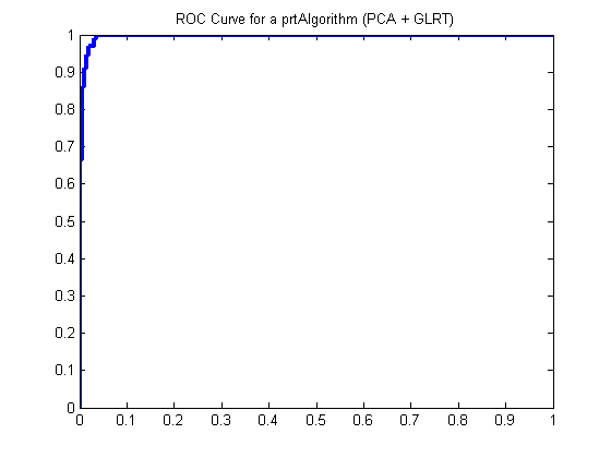
The results in the ROC curve above were generated using 10-folds cross-validation on the combination of PCA and GLRT. At each fold, 9/10ths of the data were used to train the PCA and GLRT, and 1/10th was used for evaluation.

prtAlgorithms are a very powerful tool for pattern recognition, and we hope this blog post helps clear up how to make and use them!

Let us know if you have any questions or comments.