Learning Feature Representations

Today I wanted to go through an interesting paper I recently read and show how to implement parts of that paper in the PRT. The paper is Learning Feature Representations with K-means , by Adam Coates and Andrew Y. Ng (see below for full citation).

The meat of the Coates and Ng paper deals with how to use K-means to extract meaningful dictionaries from image data. The latter part of the paper talks about how to do real machine learning with max-pooling for classification, but for today, I just wanted to introduce the MSRCORID (Microsoft Research Cambridge Object Recognition Image Database) data in the PRT and also show how to use the PRT to do some K-means dictionary learning.

The MSRCORID Database
Extracting Patches
Normalization
K-Means
Simple Bag-Of-Words Classification
Bibliography

The MSRCORID Database

For fun, I downloaded a new image database to play with for this data. The data is available for download from here: http://research.microsoft.com/en-us/downloads/b94de342-60dc-45d0-830b-9f6eff91b301/default.aspx

You can load the data automatically in the PRT, if you update to the newest version and run:

ds = prtDataGenMsrcorid;

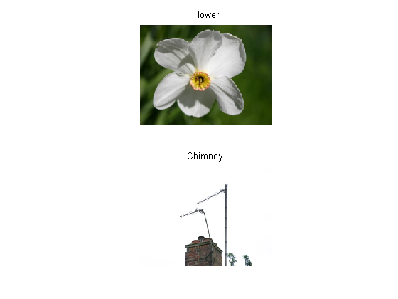
By default, that command will give a dataset with only images of chimneys and single flowers. Look at the help for prtDataGenMsrcorid to see how to load data from these, and a lot more interesting classes.

You should note that prtDataGenMsrcorid does not output a prtDataSetClass, it produces a prtDataSetCellArray. prtDataSetCellArray data objects are relatively new, and not fully documented, but they’re useful when you want to deal with datasets where each observation can have different sizes - e.g., images.

You can access elements using cell-array notation to access the .X field of the prtDataSet, for example:

subplot(2,1,1);
imshow(ds.X{1});
title('Flower');

subplot(2,1,2);
imshow(ds.X{end});
title('Chimney');

Extracting Patches

To generate a dictionary requires segmenting the initial images provided to us into sub-regions. We can acheive this by using the MATLAB function im2col which with will convert every 8x8 sub-image to a 64x1 element vector.

patchSize = [8 8];
col = [];
for imgInd = 1:ds.nObservations;

img = ds.X{imgInd};
img = rgb2gray(img);
img = imresize(img,.5);
col = cat(1,col,im2col(img,patchSize,<span class="string">'distinct'</span>)');


end
dsCol = prtDataSetClass(double(col));

Normalization

[Coates, 2012], makes it very clear that proper data normalization on a per-patch basis is fundamental to getting meaningful K-means centroids. The three main steps in the normalization are mean-normalization, energy normalization, and ZCA centering. These are all implemented in the PRT as prtPreProcZeroMeanRows, prtPreProcStdNormalizeRows, and prtPreProcZca.

As always, we can buld an algorithm out of these independent components, then train and run the algorithm on the dsCol data we created earlier:

preProc = prtPreProcZeroMeanRows + prtPreProcStdNormalizeRows(‘varianceOffset’,10) + prtPreProcZca;
preProc = preProc.train(dsCol);
dsNorm = preProc.run(dsCol);

K-Means

[Coates, 2012], makes a compelling case that K-means clustering is capable of learning dictionaries that can be easily used for classification. The K-means algorithm in Coates paper is particularly intruiging, and its very fast compared to standard K-means using euclidean distances. We’ve implemented the K-means algorithm as described in [Coates, 2012] as prtClusterSphericalKmeans, which is much faster than using the regular K-means.

skm = prtClusterSphericalKmeans(‘nClusters’,50);
skm = skm.train(dsNorm);

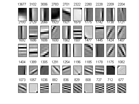
We can visualize the resulting cluster centers from the K-means processing by looking a the skm.clusterCenters, and plotting the first 50. We’ll sort these by how often data vectors were assigned to each cluster, so the top-left has the most elements, and the bottom-right has the least.



yOutK = skm.run(dsNorm);
[val,ind] = max(yOutK.X,[],2);
boolMat = zeros(size(yOutK.X));
indices = sub2ind(size(boolMat),(1:size(boolMat,1))‘,ind(:));
boolMat(indices) = 1;

clusterCounts = sum(boolMat);
[v,sortInds] = sort(clusterCounts,‘descend’);

c = skm.clusterCenters';
for i = 1:50

subplot(5,10,i);
imagesc(reshape(c(sortInds(i),:),patchSize));
title(v(i));
tickOff;


end
colormap gray

Simple Bag-Of-Words Classification

We can use some of the approaches from [Coates, 2012] to do some simple classification, also. For example, we can use our new K-means clustering algorithm to generate features for each observation. We can do this for every patch we extract from each image, but we’d like to make decisions on an image-by-image basis, so we need to aggregate over the resulting feature vectors somehow.

A clever way to do this is to use max-pooling and deep-learning as specified in [Coates, 2012], but for now we’ll just take the mean of the resulting feature vectors (in a manner similar to bag-of-words classification http://en.wikipedia.org/wiki/Bag-of-words_model )

featVec = nan(ds.nObservations,skm.nClusters);

for imgInd = 1:ds.nObservations;

img = ds.X{imgInd};
img = rgb2gray(img);
col = im2col(img,patchSize,<span class="string">'distinct'</span>);
col = double(col);
dsCol = prtDataSetClass(col');
dsCol = run(preProc,dsCol);
dsFeat = skm.run(dsCol);
feats = max(dsFeat.X,.05);
featVec(imgInd,:) = mean(feats);


end

Now we can classify our feature vectors using another classification algorithm – e.g., here we use a SVM, with ZMUV pre-processing, and max-a-posteriori classification.

dsFeat = prtDataSetClass(featVec,ds.targets);
dsFeat.classNames = ds.classNames;

yOut = kfolds(prtPreProcZmuv + prtClassLibSvm + prtDecisionMap,dsFeat,3);

close all;
prtScoreConfusionMatrix(yOut)

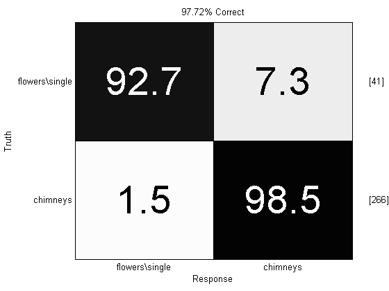
Hey! That’s not too bad for a few lines of code. At some point in the future we’ll take on the rest of the [Coates, 2012] paper, but in the meantime, let us know if you implement the max-pooling or other processes outlined therein.

Happy coding!

Note: we created prtPreProcZca, prtClusterSphericalKmeans, and prtDataGenMsrcorid for this blog entry; they’re all in the PRT, but are recent (as of 2/27/2013) so download a new version to get access to all these.

Bibliography

Adam Coates and Andrew Y. Ng, Learning Feature Representations with K-means, G. Montavon, G. B. Orr, K.-R. Muller (Eds.), Neural Networks: Tricks of the Trade, 2nd edn, Springer LNCS 7700, 2012

PRT Blog