You may have noticed in a lot of examples, we’ve made use of prtDecision objects, and might have wondered what exactly those are, and how they work. Today I’d like to describe the prtDecision* actions, and when you might want to use them.

Contents

Let’s start out with a pretty standard prtDataSet, and we’ll make a classifier and score a ROC curve:

ds = prtDataGenUnimodal;
classifier = prtClassFld;
yOutFld = kfolds(classifier,ds,3);
[pf,pd] = prtScoreRoc(yOutFld);
h = plot(pf,pd);
set(h,'linewidth',3);
title('ROC Curve for FLD');
xlabel('Pfa');
ylabel('Pd');

That ROC curve looks pretty good, but it doesn’t tell the whole story. At the end of the day, if you wanted to use your FLD algorithm in a production setting, you’ll need to make discrete decisions to take different actions depending on whether you’re calling something Class #1 or Class #0. An ROC curve is suitable for comparing performance across a range of possible operating points, but what if we wanted to know exactly what PD and PFA we were going to get for a particular decision point?

To clarify matters, let’s take a look at what the output from FLD actually looks like.

h = plot(1:yOutFld.nObservations,yOutFld.X,1:yOutFld.nObservations,yOutFld.Y);
set(h,‘linewidth’,3);
xlabel(‘Observation Index’);
legend(h,{‘FLD Output’,‘Class Label’});
title(‘FLD Output & Actual Class Label vs. Observation Index’);

The above figure shows what’s actually going on under the hood – when a classifier object is run on a data set, the output data set (yOutFld) has it’s X value set to the classifier output. In this case, the yOutFld.X value is a linear weighting of the input variables, and is shown in blue. You can see how it correlated with the actual class labels (in green).

Making Manual Decisions

Say we wanted to make decisions based on the output of the FLD. We have to choose a threshold (a point along the y-axis) such that whenever a blue data point is above the threshold, we call the output “Class 1”, and otherwise we call it “Class 0”. By visual inspection, any value between, say, 0 and 2 looks reasonable. Let’s try manually setting a threshold of 1:

yOutManual = yOutFld;
yOutManual.X = yOutManual.X > 1;
h = plot(1:yOutManual.nObservations,yOutManual.X,1:yOutManual.nObservations,yOutManual.Y);
ylim([–.1 1.1]);
set(h,‘linewidth’,3);
xlabel(‘Observation Index’);
legend(h,{‘Manual Decision Output’,‘Class Label’},4);
title(‘Manual Decision & Actual Class Label vs. Observation Index’);

You can see that our chosen threshold does pretty well. The vast majority of the time, the blue line corresponds to the green line. We can confirm this by considering the percent correct, and a confusion matrix:

prtScoreConfusionMatrix(yOutManual);
pc = prtScorePercentCorrect(yOutManual);
title(sprintf(‘Percent Correct: %.0f%%’,pc100));

98% Correct! That’s not bad. But look at what happens if we try and do the same scoring on the original output from the FLD:

prtScoreConfusionMatrix(yOutFld);
pc = prtScorePercentCorrect(yOutFld);
title(sprintf(‘Percent Correct: %.0f%% (This is clearly wrong!)’,pc100));

What happened? This is a little subtle, but whenever the PRT has to score discrete classes, like with prtScorePercentCorrect and prtScoreConfusionMatrix, it requires that the X values in the dataset to be equal to your best guess as to the real underlying class.

That worked out great for yOutManual, since we set yOutManual.X to zero for class 0, and 1 for class 1. But yOutFld has continuous values stored in it (as the earlier figure shows); you need to make discrete decisions for prtScorePercentCorrect or prtScoreConfusionMatrix to make any sense.

Decision Objects

Fortunately, the PRT provides a special kind of prtAction – prtDecisions to make those decisions for you automatically, so you can score algorithms very easily.

For example, prtDecisionBinaryMinPe tries to find a threshold based on the training data to minimize the probability of error (Pe). You can use the decision actions like you would use any other actions in a prtAlgorithm:

algo = prtClassFld + prtDecisionBinaryMinPe;
yOutDecision = kfolds(algo,ds,3);
prtScoreConfusionMatrix(yOutDecision);
pc = prtScorePercentCorrect(yOutDecision);
title(sprintf(‘Percent Correct: %.0f%%’,pc100));

Now we’re back in the ball game! You can use different decision objects to get performance at different points on the ROC curve, for example prtDecisionBinarySpecifiedPd let’s you specify a Pd to operate at:

close all;
algo = prtClassFld + prtDecisionBinarySpecifiedPd(‘pd’,.99);
yOutDecision = kfolds(algo,ds,3);
prtScoreConfusionMatrix(yOutDecision);
pc = prtScorePercentCorrect(yOutDecision);
title(sprintf(‘Percent Correct: %.0f%%’,pc100));

Note that the overall probability of error is significantly worse, but almost all of the data from Class 1 was identified as Class 1. (This may not achieve 99% Pd in some cases since the thresholds are learned differently in each fold, so there is some statistical variation in the actual Pd achieved).

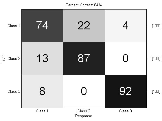
We can also use prtDecisionMap to perform multi-class decision making. The “Map” in prtDecisionMap stands for maximum a-posteriori. This basically means “decide the class corresponding to the maximum classifier output”.

ds = prtDataGenMary;
algo = prtClassKnn + prtDecisionMap;
yOutDecision = kfolds(algo,ds,3);
prtScoreConfusionMatrix(yOutDecision);
pc = prtScorePercentCorrect(yOutDecision);
title(sprintf(‘Percent Correct: %.0f%%’,pc*100));

Concluding

So, there you go! prtDecision objects handle a lot of book-keeping internally, so that you don’t generally have to worry about making sure to keep class names and indices straight. We recommend using them instead of manually making your own decision functions to operate on output classes.

As always, please feel free to comment or e-mail us with questions or ideas.