The MNIST Database (http://yann.lecun.com/exdb/mnist/) is a very well-known machine learning dataset consisting of a few thousand instances of handwritten digits from 0-9. MNIST is actually a subset of a larger NIST database, but the authors (see the linked page above) were kind enough to do some basic pre-processing of MNIST for us. MNIST was for a long time very widely used in the ML literature as an example of an easy to use real data set to evaluate new ideas.
Contents
Obtaining, Loading, and Visualizing MNIST Data
Tools to read in the MNIST database into the PRT are available in the newest PRT version. To conserve bandwidth, the actual MNIST data isn’t included in the PRT (it would kill our subversion servers). Instead you can download the MNIST database from the website linked above. Once you’ve downloaded it, extract the data into:
fullfile(prtRoot,'dataGen','dataStorage','MNIST') %MATLAB command will tell you the directory
ans =

C:\Users\Pete\Documents\MATLAB\toolboxes\nfPrt\dataGen\dataStorage\MNIST
For example, on my system:
ls(fullfile(prtRoot,'dataGen','dataStorage','MNIST'))
.                        t10k-labels.idx1-ubyte
..                       train-images.idx3-ubyte
t10k-images.idx3-ubyte   train-labels.idx1-ubyte
Once the MNIST files are in the right place, execute the PRT command:
dsTrain = prtDataGenMnist;
to extract the data. ( Note, prtDataGenMnist makes use of a M-file function called readMNIST by Siddharth Hegde. It’s available from: http://www.mathworks.com/matlabcentral/fileexchange/27675-read-digits-and-labels-from-mnist-database ).
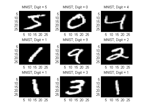
Once loaded, we can use a number of different tools to visualize the data. First, let’s visualize the data as images. We know that the images are size 28x28, but since the prtDataSetClass object expects each observation to correspond to a 1xN vector, we store all the 28x28 images as 1x784 vectors.
imageSize = [28 28];

for i = 1:9;
    subplot(3,3,i);
    x = dsTrain.getX(i); %1x784
    y = dsTrain.getY(i);
    imagesc(reshape(x,imageSize));
    colormap gray;
    title(sprintf('MNIST; Digit = %d',y));
end
Classification: PLSDA
What kinds of classification approaches can we apply to this data set? We need to satisfy a few requirements: 1) M-Ary classification, 2) Relatively fast, 3) Relatively insensitive to a large number of dimensions (784 dimensional vectors). One particularly fast, linear approach to classification that’s relatively insensitive to the number of feature dimensions is partial-least squares discriminant analysis, implemented in the PRT as prtClassPLSDA. With only a few lines of code we can implement and evaluate a PLSDA classifier on the MNIST data, for example:
algo = prtClassPlsda(‘nComponents’,20) + prtDecisionMap; %we include the Max-A-Posteriori classifier
yOut = algo.kfolds(dsTrain,3); %3 folds x-val
pc = prtScorePercentCorrect(yOut);
subplot(1,1,1);
prtScoreConfusionMatrix(yOut);
title(sprintf(‘3-Fold X-Val PLSDA on 10,000 MNIST Database Train Samples; %.0f%% Correct’,pc*100));
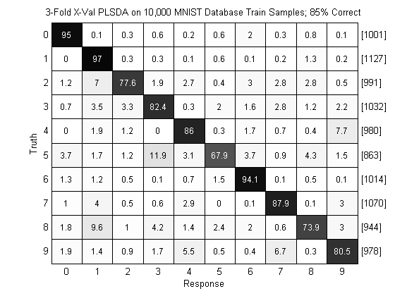
This basic example results in the above figure, where we see we’ve achieved about 84% correct classification, and we can analyze confusions between digits. For example, the digits 4 and 9 are often confused, which seems intuitive since they look relatively similar.
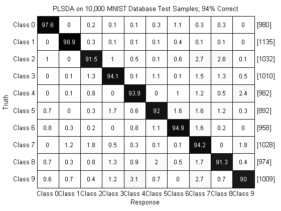
We can also evaluate the PLSDA classifier trained on 10,000 training points and evaluated on the MNIST testing data. To do so we first load the testing data, then train our classifier and evaluate it:
dsTest = prtDataGenMnistTest;
algo = algo.train(dsTrain);
yOut = algo.run(dsTest);
pc = prtScorePercentCorrect(yOut);
subplot(1,1,1);
prtScoreConfusionMatrix(yOut);
title(sprintf('PLSDA on 10,000 MNIST Database Test Samples; %.0f%% Correct',pc*100));
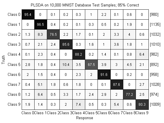
Performance on the test set is relatively similar to performance in cross-validation as can be seen above.
Overall, our performance is hovering around a 15% error rate. That’s roughly comparable to the 12% error reported in LeCun et al., 1988, and here we’re not using a lot of the techniques in the Le Cun paper (and this is with barely 5 lines of code!).
Classification: SVM
As the results on http://yann.lecun.com/exdb/mnist/ illustrate, other approaches to digit classification have done much better than our simple PLSDA classifier. We can use the PRT to apply more complicated classifiers to the same data also, and hopefully decrease our error rate.
For example, consider a simple application of an SVM classifier to the digit recognition problem. Since the SVM is not an M-ary classification technique, we need to wrap our SVM in a One-Vs-All classifier to perform M-ary classification (Warning: the following code took about 30 minutes to run on my laptop):
marySvm = prtPreProcZmuv + prtClassBinaryToMaryOneVsAll(‘baseClassifier’,prtClassLibSvm) + prtDecisionMap;
yOut = marySvm.kfolds(dsTrain,3);
pc = prtScorePercentCorrect(yOut);
subplot(1,1,1);
prtScoreConfusionMatrix(yOut);
title(sprintf(‘3-Fold X-Val SVM on 10,000 MNIST Database Train Samples; %.0f%% Correct’,pc*100));
Warning: Non-finite or zero standard deviation encountered.  Replacing invalid
standard deviations with 1
Warning: Non-finite or zero standard deviation encountered.  Replacing invalid
standard deviations with 1
Warning: Non-finite or zero standard deviation encountered.  Replacing invalid
standard deviations with 1
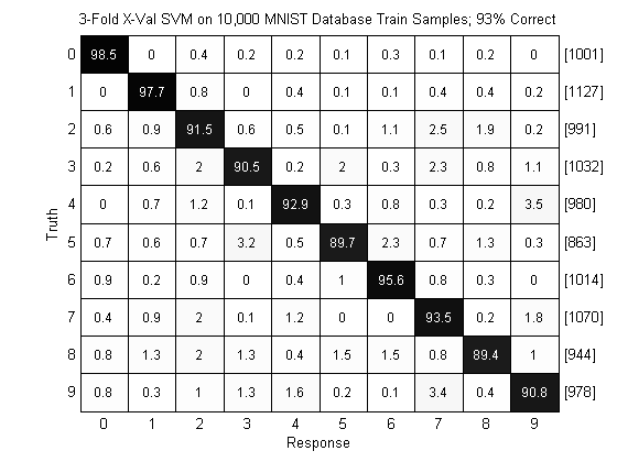
As can be seen above, the SVM achieves an error rate of 5% on this data set! That’s a significant improvement over the PLSDA classification we showed before. Similarly to with PLSDA, we can also evaluate the algorithm on completely separate testing data:
marySvm = marySvm.train(dsTrain);
yOut = marySvm.run(dsTest);
pc = prtScorePercentCorrect(yOut);
subplot(1,1,1);
prtScoreConfusionMatrix(yOut);
title(sprintf('PLSDA on 10,000 MNIST Database Test Samples; %.0f%% Correct',pc*100));
Warning: Non-finite or zero standard deviation encountered.  Replacing invalid
standard deviations with 1
And we see that performance is comparable to the cross-validated results. (Note that more advanced applications of SVM classifiers can do even better than the results reported here – Le Cun et al., 1998 reported 1.4% error rates with an SVM and some additional processing).
Exploring the Results
If we wanted to improve classification, we could optimize over the SVM parameters, kernel, pre-processing etc. But before we did that, it might be instructive to investigate what digits the SVM classifier is mislabeling, and see if some of them seem like reasonable mistakes to make. The following code will pick 9 instances where the SVM output label was different from the actual data label, and plot them in a subplot.
incorrect = find(yOut.getX ~= yOut.getY);
yOutTestMisLabeled = yOut.retainObservations(incorrect);
dsTestMisLabeled = dsTest.retainObservations(incorrect);
for i = 1:9; %dsTestMisLabeled.nObservations;
      randWrong = ceil(rand*dsTestMisLabeled.nObservations); %pick a random wrong element
      subplot(3,3,i);
      x = dsTestMisLabeled.getX(randWrong);
      img = reshape(x,imageSize);
      imagesc(img);
      colormap gray;

title(sprintf('Actual: %d; SVM Label: %d',yOutTestMisLabeled.getY(randWrong),yOutTestMisLabeled.getX(randWrong)));
end
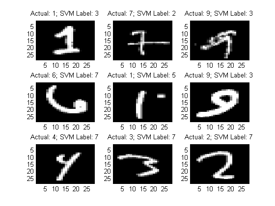
Visual inspection of these mistakes illustrate some of the causes of confusions in the SVM. For example, highly slanted digits are often mis-labeled. Mitigating some of these mistakes may require significantly more than simply optimizing SVM parameters!
Interested readers can refer to a large body of literature that has previously investigated this data set (http://yann.lecun.com/exdb/mnist/) for tips, tricks, and ideas for further improving performance on this data set. One particularly exciting recent advance is based on Hinton’s deep learning networks, which enables very efficient learning on the MNIST database www.cs.toronto.edu/~hinton/science.pdf).
We hope this example shows how quickly you can get from data to results with the PRT. Please let us know if you have comments or questions!