Hi everyone, Today we’ll talk about a new clustering algorithm in the PRT - Mean-Shift clustering. Mean shift clustering is widely used in image processing, and has a few nice properties - for example, it’s not necessary to specify ahead of time how many clusters you need. Instead you specify a clustering bandwidth. We’ll show some examples below. If you want a good introduction to mean-shift clustering, see the wiki page.

Note, unlike most of our other objects, prtClusterMeanShift requires the bio-informatics toolbox,

Contents

prtClusterMeanShift

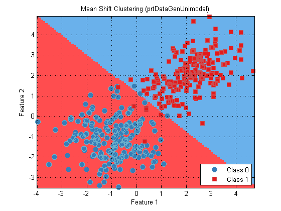
As you might expect, we start by generating some data, and a prtClusterMeanShift object:

ds = prtDataGenUnimodal;
ms = prtClusterMeanShift;

We can train, run, and plot the mean-shift algorithm just like anything else

ms = ms.train(ds);
plot(ms);

Bandwidth

In the above figure, the mean-shift algorithm correctly identified two clusters. We can mess with the Gaussian bandwidth parameter (sigma) to see how this affects how many clusters mean-shift finds:

sigmaVec = [.1 .3 .6 1 2 5];
for ind = 1:length(sigmaVec)


ms = prtClusterMeanShift;
ms.sigma = sigmaVec(ind);
ms = ms.train(ds);

subplot(2,3,ind);
plot(ms);
prtPlotUtilFreezeColors
title(sprintf(<span class="string">'sigma = %.2d'</span>,sigmaVec(ind)));


end

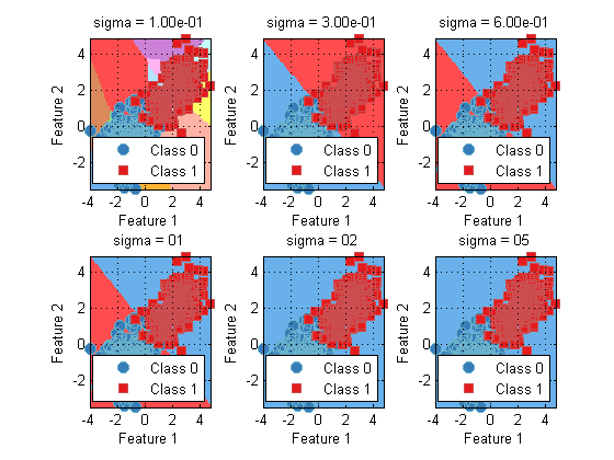
Note how changing the sigma value can drastically alter the number of clusters that mean-shift finds. Careful tuning of that parameter may be necessary for your particular application.

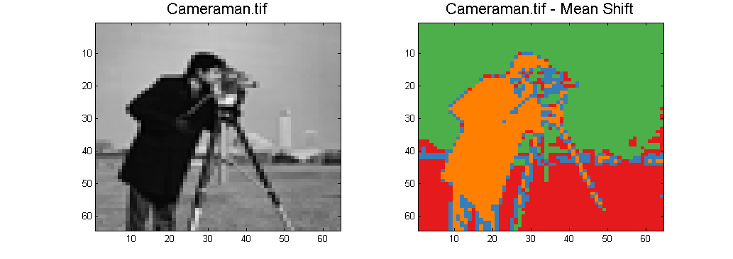
Application to Images

We mentioned before that you can use mean shift in image processing – here’s a quick and dirty example applying mean shift to the famous “cameraman” photo:

I = imread(‘cameraman.tif’);
I = imresize(I,0.25);
I = double(I);
[II,JJ] = meshgrid(1:size(I,2),1:size(I,1));


ij = bsxfun(@minus,cat(2,II(:),JJ(:)),size(I));

ds = prtDataSetClass(cat(2,I(:)-128,ij));
ms = train(prtClusterMeanShift(‘sigma’,200),ds);
out = run(ms, ds);
[~,out] = max(out.X,[],2);

figure(‘position’,[479 447 1033 366]);
subplot(1,2,1)
imagesc(I)
colormap(gray(256))
prtPlotUtilFreezeColors;
title(‘Cameraman.tif’,‘FontSize’,16);

subplot(1,2,2);
imagesc(reshape(out,size(I)));
colormap(prtPlotUtilClassColors(ms.nClusters))
prtPlotUtilFreezeColors;
title(‘Cameraman.tif – Mean Shift’,‘FontSize’,16);

Determining Stopping

Determining convergence in a mean shift scenario can actually be pretty subtle, the code we provide is based on

http://dl.acm.org/citation.cfm?id=1143864 Fast Nonparametric Clustering with Gaussian Blurring Mean-Shift Miguel A. Carreira-Perpinan ICML 2006

Conclusion

That’s all for now. If you have the bio-informatics toolbox, have fun with prtClusterMeanShift. If you don’t, we need to find or write a replacement for graphconncomp to de-couple MeanShift from bioinformatics. One day, hopefully.