Today I’d like to give a quick tour of how to use PCA in the PRT to easily reduce the dimensionality of your data set in a meaningful, principled way.

Contents

Introduction & Theory

Principal component analysis (PCA) is a widely used technique in the statistics and signal processing literature. Even if you haven’t heard of PCA, if you know some linear algebra, you may have heard of the singular value decomposition (SVD), or, if you come from the signal processing literature, you’ve probably heard of the Karhunen–Loeve transformation (KLT). Both of these are identical in form to PCA. Turns out a lot of different groups have re-created the same algorithm in a lot of different fields!

We won’t have time to delve into the nitty gritty about PCA here. For our purposes it’s enough to say that given a (zero-mean) data set X of nObservations x nFeatures, we often want to find a linear transformation of X, S = X*Z, for a matrix Z of size nPca x nFeatures where:

1) nPca < nFeatures
2) The resulting data, S, contains "most of the information from" X.

As you can imagine, the phrase “most of the information” is vague, and subject to interpretation… Mathematically, PCA considers “most of the information in X” to be equivalent to “explains most of the variance in X. It turns out that this statement of the problem has some very nice mathematical solutions - e.g., the columns of S can be viewed as the dominant eigenvectors in the covariance of X!

You can find our more about PCA on the fabulous wikipedia article: https://en.wikipedia.org/wiki/Principal_component_analysis.

In the PRT

PCA is implemented in the PRT using prtPreProcPca. Older versions of prtPreProcPca used to make use of different algorithms for different sized data sets (there are a lot of ways to do PCA quickly depending on matrix dimensions). Since 2012, we found that the MATLAB function SVDS was beating all of our approaches in terms of speed and accuracy, so have switched over to using SVDS to solve for the principal component vectors.

Let’s take a quick look at some PCA projections. First, we’ll need some data:

ds = prtDataGenUnimodal;

We also need to make a prtPreProcPca object, and we’ll use 2 components in the PCA projection:

pca = prtPreProcPca('nComponents',2);

prtPreProc* objects can be trained and run just like any other objects:

pca = pca.train(ds);

Let’s visualize the results, first we’ll look at the original data, and the vectors from the PCA analysis:

plot(ds);
hold on;
h1 = plot([0 pca.pcaVectors(1,1)],[0,pca.pcaVectors(2,1)],'k');
h2 = plot([0 pca.pcaVectors(1,2)],[0,pca.pcaVectors(2,2)],'k--');
set([h1,h2],'linewidth',3);
hold off;
axis equal;
title('Original Data & Two PCA Vectors');

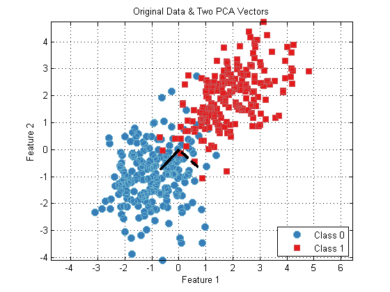
From this plot, we can see that the PCA vectors are oriented first along the dimension of largest variance in the data (diagonal wiht a positive slope), and the second PCA is oriented orthogonal to the first PCA.

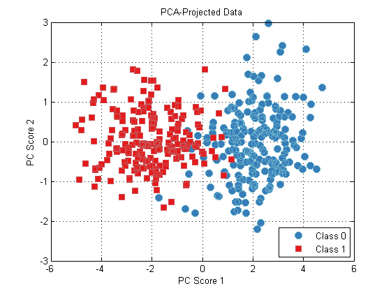
We can project our data onto this space using the RUN method:

dsPca = pca.run(ds);
plot(dsPca);
title(‘PCA-Projected Data’);

How Many Components?

In general, it might be somewhat complicated to determine how many PCA components are necessary to explain most of the variance in a particular data set. Above we used 2, but for higher dimensional data sets, how many should we use in general?

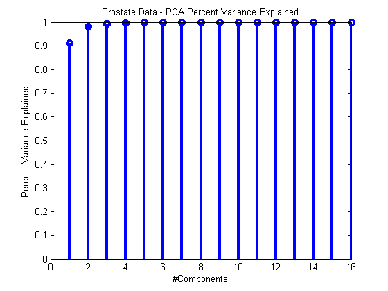
We can measure how much variance each PC explains during training by exploring the vector pca.totalPercentVarianceCumulative which is set during training. This vector contains the percent of the total variance of the data set explained by 1:N PCA components. For example, totalPercentVarianceCumulative(3) contains the percent variance explained by components 1 through 3. When this metric plateaus, that’s a pretty good sign that we have enough components.

For example:

ds = prtDataGenProstate;
pca = prtPreProcPca(‘nComponents’,ds.nFeatures);
pca = pca.train(ds);


stem(pca.totalPercentVarianceCumulative,‘linewidth’,3);
xlabel(‘#Components’);
ylabel(‘Percent Variance Explained’);
title(‘Prostate Data – PCA Percent Variance Explained’);

Normalization

For PCA to be meaningful, the data used has to have zero-mean columns, and prtPreProcPca takes care of that for you (so you don’t have to zero mean the columns yourself). However, different authors disagree about whether or not the columns provided to PCA should all have the same variance before PCA analysis. Depending on normalization, you can get very different PCA projections. To leave the option open, the PRT does not automatically normalize the columns of the input data to have uniform variance. You can manually enforce this before your PCA processing with prtPreProcZmuv.

Here’s a simplified example, where we do the two processes separately to show the differences.

ds = prtDataGenProstate;
dsNorm = rt(prtPreProcZmuv,ds);
pca = prtPreProcPca(‘nComponents’,ds.nFeatures);
pca = pca.train(ds);
pcaNorm = pca.train(dsNorm);


subplot(2,1,1);
stem(pca.totalPercentVarianceCumulative,‘linewidth’,3);
xlabel(‘#Components’);
ylabel(‘Percent Variance Explained’);
title(‘Prostate Data – PCA Percent Variance Explained’);

subplot(2,1,2);
stem(pcaNorm.totalPercentVarianceCumulative,‘linewidth’,3);
xlabel(‘#Components’);
ylabel(‘Percent Variance Explained’);
title(‘Prostate Data – PCA Percent Variance Explained (Normalized Data)’);

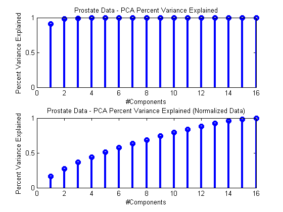
As you can see, processing normalized and un-normalized data results in quite different assessments of how many PCA components are required to summarize the data.

Our recommendation is that if your data comes from different sources, with different sensor ranges or variances (as in the prostate data), it’s imperative that you perform standard-deviation normalization prior to PCA processing.

Otherwise, it’s worthwhile to try both with and without ZMUV pre-processing and see what gives better performance.

Conclusion

That’s about it for PCA processing. Of course, you can use PCA as a pre-processor for any algorithm you’re developing, to reduce the dimensionality of your data, for example:

algo = prtPreProcPca + prtClassLibSvm;

Let us know if you have questions or comments about using prtPreProcPca.