A few weeks ago we took a look at a paper by Coates and Ng that dealt with learning feature representations for image processing and classification. (See: this). Today I want to take a second look at that paper, and especially what they mean by max-pooling over regions of the image.
Contents
The MSRCORID Database
If you have already read through our previous post, you know how to get the Microsoft Research Cambridge Object Recognition Image Database (MSRCORID), which is really a fantastic resource for image processing and classification.
Once you’ve downloaded, we can run the following code which was for the most-prt ripped right out of the previous blog post:
ds = prtDataGenMsrcorid;

patchSize = [8 8];
col = [];
for imgInd = 1:ds.nObservations;
    img = ds.X{imgInd};
    img = rgb2gray(img);
    img = imresize(img,.5);
    col = cat(1,col,im2col(img,patchSize,'distinct')');
end
dsCol = prtDataSetClass(double(col));

preProc = prtPreProcZeroMeanRows + prtPreProcStdNormalizeRows('varianceOffset',10) + prtPreProcZca;
preProc = preProc.train(dsCol);
dsNorm = preProc.run(dsCol);

skm = prtClusterSphericalKmeans('nClusters',50);
skm = skm.train(dsNorm);
Max-Pooling
Last time, we used a simple bag-of-words model to do classification based on the feature vectors in each image. That’s definitely an interesting way to proceed, but most image-processing techniques make use of something called “max-pooling” to aggregate feature vectors over small regions of an image.
The process can be accomplished in MATLAB using blockproc.m, which is in the Image-processing toolbox. (If you don’t have image processing, it’s not too hard to write a replacement for blockproc.)
The goal of max-pooling is to aggregate feature vectors over local regions of an image. For example, we can take the MAX of the cluster memberships over each 8x8 region in an image using something like:
featsBp = blockproc(feats,[8 8],@(x)max(max(x.data,[],1),[],2));
Where we’ve assumed that feats is size nx x ny x nFeats.
Max pooling is nice because it reduces the dependency of the feature vectors on their exact placement in an image (each element of each 8x8 block gets treated about the same), and it also maintains a lot of the information that was in each of the feature vectors, especially when the feature vectors are expected to be sparse (e.g., have a lot of zeros; see http//www.ece.duke.edu/~lcarin/Bo12.3.2010.ppt).
There’s a lot more to max-pooling than we have time to get into here, for example, you can max-pool, and then re-cluster, and then re-max-pool! This is actually a super clever technique to reduce the amount of spatial variation in your image, and also capture information about the relative placements of various objects.
featVec = nan(ds.nObservations,skm.nClusters*20);
clusters = skm.run(dsNorm);

for imgInd = 1:ds.nObservations;
    img = ds.X{imgInd};
    img = rgb2gray(img);
    imgSize = size(img);

    % Extract the sub-patches
    col = im2col(img,patchSize,'distinct');
    col = double(col);
    dsCol = prtDataSetClass(col');
    dsCol = run(preProc,dsCol);
    dsFeat = skm.run(dsCol);
    dsFeat.X = max(dsFeat.X,.05);

    % Max Pool!
    %   Feats will be size 30 x 40 x nClusters
    %   featsBp will be size [4 x 5] x nClusters (because of the way
    %   blockproc handles edsges)
    feats = reshape(dsFeat.X,imgSize(1)/8,imgSize(2)/8,[]);
    featsBp = blockproc(feats,[8 8],@(x)max(max(x.data,[],1),[],2));

    % We'll cheat a little here, and use the whole max-pooled feature set
    % as our feature vector.  Instead, we might want to re-cluster, and
    % re-max-pool, and repeat this process a few times.  For now, we'll
    % keep it simple:
    featVec(imgInd,:) = featsBp(:);
end
Now that we’ve max-pooled, we can use our extracted features for classification - we’ll use a simple PLSDA + MAP classifier and decision algorithm here:
dsFeat = prtDataSetClass(featVec,ds.targets);
dsFeat.classNames = ds.classNames;

yOut = kfolds(prtClassPlsda + prtDecisionMap,dsFeat,3);

close all;
prtScoreConfusionMatrix(yOut)
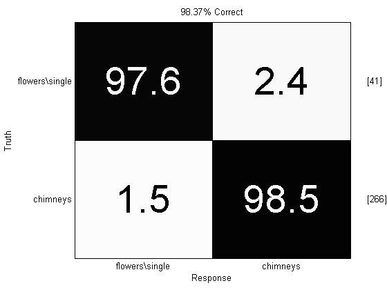
Almost 99% correct! We’ve improved performance over our previous work with bag-of-words models, and an SVM, by just (1) max-pooling, and (2) replacing the SVM with a PLSDA classifier.
Multiple Classes
Until now we’ve focused on just two classes in MSRCORID. But there are a lot of types of objects in the MSRCORID database. In the following, we just repeat a bunch of the code from above, and run it on a data set containing images of benches, buildings, cars, chimneys, clouds and doors:
ds = prtDataGenMsrcorid({‘benches_and_chairs’,‘buildings’,‘cars\front view’,‘cars\rear view’,‘cars\side view’,‘chimneys’,‘clouds’,‘doors’});

patchSize = [8 8];
col = [];
for imgInd = 1:ds.nObservations;

img = ds.X{imgInd};
img = rgb2gray(img);
img = imresize(img,.5);
col = cat(1,col,im2col(img,patchSize,<span class="string">'distinct'</span>)');


end
dsCol = prtDataSetClass(double(col));

preProc = prtPreProcZeroMeanRows + prtPreProcStdNormalizeRows(‘varianceOffset’,10) + prtPreProcZca;
preProc = preProc.train(dsCol);
dsNorm = preProc.run(dsCol);

skm = prtClusterSphericalKmeans(‘nClusters’,50);
skm = skm.train(dsNorm);

featVec = nan(ds.nObservations,skm.nClusters*20);
clusters = skm.run(dsNorm);

for imgInd = 1:ds.nObservations;

img = ds.X{imgInd};
img = rgb2gray(img);
imgSize = size(img);

<span class="comment">% Extract the sub-patches</span>
col = im2col(img,patchSize,<span class="string">'distinct'</span>);
col = double(col);
dsCol = prtDataSetClass(col');
dsCol = run(preProc,dsCol);
dsFeat = skm.run(dsCol);
dsFeat.X = max(dsFeat.X,.05);

<span class="comment">% Max Pool!</span>
<span class="comment">%   Feats will be size 30 x 40 x nClusters</span>
<span class="comment">%   featsBp will be size [4 x 5] x nClusters (because of the way</span>
<span class="comment">%   blockproc handles edsges)</span>
feats = reshape(dsFeat.X,imgSize(1)/8,imgSize(2)/8,[]);
featsBp = blockproc(feats,[8 8],@(x)max(max(x.data,[],1),[],2));

<span class="comment">% We'll cheat a little here, and use the whole max-pooled feature set</span>
<span class="comment">% as our feature vector.  Instead, we might want to re-cluster, and</span>
<span class="comment">% re-max-pool, and repeat this process a few times.  For now, we'll</span>
<span class="comment">% keep it simple:</span>
featVec(imgInd,:) = featsBp(:);


end

dsFeat = prtDataSetClass(featVec,ds.targets);
dsFeat.classNames = ds.classNames;

yOut = kfolds(prtClassPlsda(‘nComponents’,10) + prtDecisionMap,dsFeat,3);
yOut.classNames = cellfun(@(s)s(1:min([length(s),10])),yOut.classNames,‘uniformoutput’,false);
close all;
prtScoreConfusionMatrix(yOut);
set(gcf,‘position’,[426   125   777   558]);
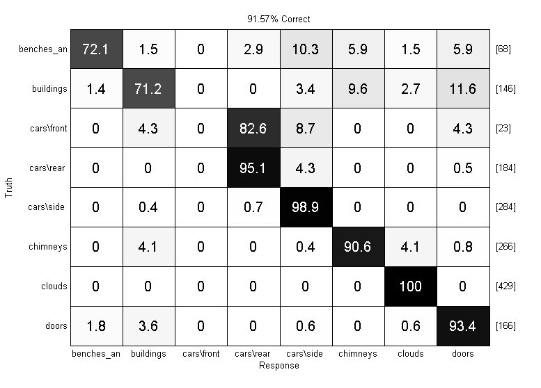
Now we’re doing some image processing! Overall we got about 90% correct, and that includes a lot of confusions between cars\front and cars\rear. That makes sense since the front and backs of cars look pretty similar, and there are only 23 car front examples in the whole data set.
Conclusions
The code in a lot of this blog entry is pretty gross – for example we have to constantly be taking data out of, and putting it back into the appropriate image sizes.
At some point in the future, we’d like to introduce a good prtDataSet that will handle cell-arrays containing images properly. We’re not there yet, but when we are, we’ll let you know on this blog!
Happy coding!
Bibliography
Adam Coates and Andrew Y. Ng, Learning Feature Representations with K-means, G. Montavon, G. B. Orr, K.-R. Muller (Eds.), Neural Networks: Tricks of the Trade, 2nd edn, Springer LNCS 7700, 2012