Today I’d like to take a look at using a particular approach to feature selection in the PRT, and how that can be used to perform dimension reduction. The approach we’ll use is called “sequential forward search”, and is implemented in prtFeatSelSfs.
Contents
Some Data
The PRT comes with a utility function to generate data that has about 10 features, and for which only 5 of the features are actually informative. The function is prtDataGenFeatureSelection, I’ll let the help entry explain how it works:
help prtDataGenFeatureSelection
 prtDataGenFeatureSelection   Generates some unimodal example data for the prt.
   DataSet = prtDataGenFeatureSelection
   The data is distributed:
        H0: N([0 0 0 0 0 0 0 0 0 0],eye(10))
        H1: N([0 2 0 1 0 2 0 1 0 2],eye(10))

  Syntax: [X, Y] = prtDataGenFeatureSelection(N)

  Inputs:
        N ~ number of samples per class (200)

  Outputs:
    X - 2Nx2 Unimodal data
    Y - 2Nx1 Class labels

  Example:
    DataSet = prtDataGenFeatureSelection;
    explore(DataSet)

  Other m-files required: none
  Subfunctions: none
  MAT-files required: none

  See also: prtDataGenUnimodal
As you can see from the help, only dimensions 2, 4, 6, 8, and 10 are actually informative in this data set. And we can use feature selection to help us pick out what features are actually useful.
Feature Selection
Feature selection objects are prefaced in the prt with prtFeatSel*, and they act just like any other prtAction objects. During training a feature selection action will typically perform some iterative search over the feature space, and determine which features are most informative. At run-time, the same object will return a prtDataSet containing onlt the features the algorithm considered “informative”.
For example:
ds = prtDataGenFeatureSelection;
featSel = prtFeatSelSfs;
featSel = featSel.train(ds);
dsFeatSel = featSel.run(ds);

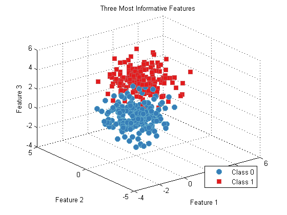
plot(dsFeatSel);
title('Three Most Informative Features');

Defining “Informative”
How does the feature selection algorithm determine what features are informative? For many (but not necessarily all) feature selection objects, the interesting field is “evaluationMetric”.
Let’s take a look:
featSel.evaluationMetric
ans =@(DS)prtEvalAuc(prtClassFld,DS)
Obviously, evaluationMetric is a function handle – in particular it represents a call to a prtEval method. prtEval methods typically take 2 or 3 input arguments – a classifier to train and run, a data set to train and run on, and (optionally) a number of folds (or fold specification) to use for cross-validation.
Feature selection objects iteratively search through the features available – in this case, all 10 of them, and apply the prtEval* method to the sub-sets of data formed by retaining a sub-set of the available features. The exact order in which the features are retained and removed depends on the feature selection approach – in SFS, the algorithm first iteratively searches through the features – 1,2,3…,10. Then it remembers which single feature provided the best performance – say it was feature 2. Next, the SFS algorithm iteratively searches through all 9 combinations of other features with feature 2: { {1,2},{3,2},{4,2},…,{10,2}} And remembers which of those performed best. This process is iterated, and features continually added to the set being evaluated until nFeatures are selected.
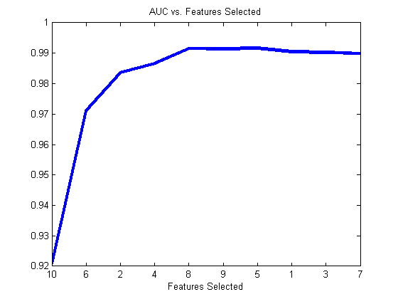
The resulting performance is then stored in “performance”, and the features selected are stored in “selectedFeatures”. Let’s force the SFS approach to look for 10 features (so it will eventually select all of them).
ds = prtDataGenFeatureSelection; featSel = prtFeatSelSfs; featSel.nFeatures = ds.nFeatures; featSel.evaluationMetric = @(DS)prtEvalAuc(prtClassFld,DS,3); featSel = featSel.train(ds);h = plot(1:ds.nFeatures,featSel.performance); set(h,‘linewidth’,3); set(gca,‘xtick’,1:ds.nFeatures); set(gca,‘xticklabel’,featSel.selectedFeatures); xlabel(‘Features Selected’); title(‘AUC vs. Features Selected’);

The features that get selected tend to favor features 2,6, and 10, then features 4 and 8, which makes sense as these are the 3 most informative followed by the two moderately-informative features!
Conclusions
There are a number of prtFeatSel actions available, but not as many as we’d like. We’re constantly on the look-out for new ones, and we’d like to one day include “K-forward, L-Backward” searches, but just haven’t had the time recently.
Also, this example only used prtEvalAuc as the performance metric, but there are a number of prtEval functions you can use, or, of course – feel free to write your own!
Take a look at prtEvalAuc to see how they work and how to create your own!
Enjoy!