In part 1 we talked about how use RVs to change the statistical model used by prtClassMap so that we can flexibly model the data. If you recall we can set the “rvs” property to correspond to prtRvMvn to model the data using multi-variate normal distributions or we can set it some other value to change the resulting model and thus the classifier. Now, we are going to talk about how we can make probabilistic mixtures in much the same way.
Contents
Mixture Models
In general, the term “mixture model” implies that each observation of data has an associated hidden variable and that observation is drawn from a distribution that is dependent on that hidden variable. In general statistics, a mixture model can have either continuous or discrete hidden variables. In the PRT, our prtRvMixture only considers discrete mixtures. That is, there are fixed number of “components” each with a mixing proportion and each component is itself a parameterized distribution, like a Gaussian.
The most common mixture is the Gaussian mixture model (GMM). A guassian mixture model with K components has a K dimensional discrite distrubtion for the mixing variable and has K individual Gaussian components. Today’s post will focus on using working with Gaussian mixture models.
prtRvMixture
prtRvMixture has two main properties that are of interest “components” and “mixingProportions”.
components should be an array of prtRvs that also inherit from prtRvMembershipModel. Without getting too indepth a prtRvMembershipModel is a special attribute of some prtRvs that specifies that this RV knows how to work inside of a mixture model. As we mentioned before, we are focusing on mixture of prtRvMvn objects to make a Gaussian mixture model. Luckily prtRvMvn inherits from prtRvMembershipModel and therefore it knows how to work in a mixture.
mixingProportions is the discrite mixing density for the mixture model. It should be a vector that sums to one with the same length as the “components” array.
To get started let’s make an array of 2D MVN RV objects with different means and a non-diagonal covariance matrix.
gaussianSet1 = repmat(prtRvMvn('sigma',[1 -0.5; -0.5 2;]),2,1);
gaussianSet1(1).mu = [-2 -2];
gaussianSet1(2).mu = [2 2];
Then we will can make a mixture by specifying some mixingProportions
mixture1 = prtRvMixture('components',gaussianSet1,'mixingProportions',[0.5 0.5]);
Because prtRvMixtures are prtRvs we get all of the nice plotting that comes along with things. Let’s take a look at the density of our prtRv
plotPdf(mixture1);

To show how we can do classification with these mixtures, let’s make another mixture with different parameters. Then we will draw some data from both mixtures and plot our classification dataset.
gaussianSet2 = repmat(prtRvMvn(‘sigma’,[1 0.5; 0.5 3;]),2,1); gaussianSet2(1).mu = [2 -2]; gaussianSet2(2).mu = [-2 2];mixture2 = prtRvMixture(‘components’,gaussianSet2,‘mixingProportions’,[0.5 0.5]);
ds = prtDataSetClass( cat(1,mixture1.draw(500),mixture2.draw(500)), prtUtilY(500,500)); % Draw 500 samples from each mixture plot(ds)
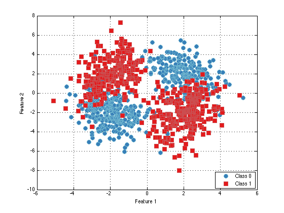
Using prtRvMixtures for Classification
Like we showed in part 1 of this series we can set the “rvs” property of prtClassMap to any prtRv object and use that rv for classification. Let’s for prtClassMap to use a mixture of prtRvMvn objects.
emptyMixture = prtRvMixture(‘components’,repmat(prtRvMvn,2,1)); % 2 component mixtureclassifier = prtClassMap(‘rvs’,emptyMixture);
trainedClassifier = train(classifier, ds);
plot(trainedClassifier);
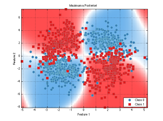
As you can see it looks like this classifier would perform quite well. We can see that the learned means of the class 0 data (blue) closely match the means that we specified above for guassianSet1. So things appear to be working well.
cat(1,trainedClassifier.rvs(1).components.mu)
ans = -1.9712 -2.04882.0139 1.9548
prtRvGmm
Since Guassian mixture models are the most common type of mixture a number of techniques have been established that help them perform better when working with limited and/or high dimensional data. To help facilitate some of those tweak there is prtRvGmm. It works much the same way as prtRvMixture only the components must be prtRvMvns.
mixture1Gmm = prtRvGmm(‘components’,gaussianSet1,‘mixingProportions’,[0.5 0.5]);plotPdf(mixture1Gmm);
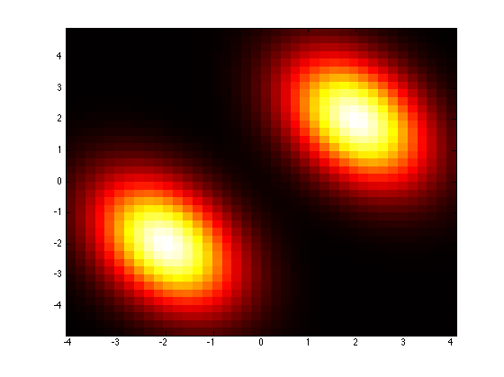
One of the available tweaks is that the covarianceStructure of all components is controled by a single parameter, “covarianceStructure’. See the documentation prtRvMvn to know how this works. Let’s see how changing the covarianceStructure of all of our components changes the appears of our density.
mixture1GmmMod = mixture1Gmm; mixture1GmmMod.covarianceStructure = ‘spherical’; % Force independence with a shared variance.plotPdf(mixture1GmmMod);
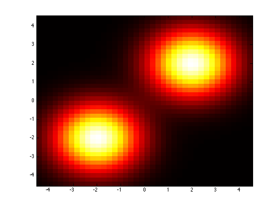
Using prtRvGmm for classification
Using prtRvGmm for classification is a little easier than prtRvMixture because we only need to specify the number of components. We don’t have to built the array of components ourselves.
Let’s redo the same problem as before.
classifier = prtClassMap(‘rvs’,prtRvGmm(‘nComponents’,2));
trainedClassifier = train(classifier,ds);
plot(trainedClassifier);

As you can see, things look nearly identical (as they should). Now, let’s make use of a few of the extra tweak offered by prtRvGmm and see how they change our decision contours.
classifier = prtClassMap(‘rvs’,prtRvGmm(‘nComponents’,2,‘covarianceStructure’,‘spherical’,‘covariancePool’,true));
trainedClassifier = train(classifier,ds);
plot(trainedClassifier);
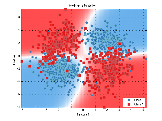
You can see that the decision contours are more regular now. This may help classificaiton performance in the precense of limited and/or high dimensional data.
Conclusions
We hope this post showed how you can use mixture models just like any other prtRv object when doing classificaiton using prtClassMap.
Chances are that you want to use prtRvGmm for your mixture modeling needs but you might be able to guess that prtRvMixture is much more general allowing you to make mixture models out of general prtRvs. However, at this time the only prtRv that is able to be used is prtRvMvn. We are interested in making more prtRvs compatible but we want to know what people want to use. Let us know if you need something specific.
In the next part of this series we will look at prtRvHmm and how it can be used for time-series classification.