People are often asking us why we don’t have a neural-network (NNET) implemented in the PRT. Formerly, we never focused on making a home-grown NNET object, since the MathWorks already has a (neural network toolbox), and often we’ve found that NNET results aren’t significantly better than other classifiers, and they can be difficult to train. That said, neural network classifiers can provide good results, some recent advances in deep-learning have brought NNET classifiers back into vogue, and they’re often fun to play with. As a result, we’ve finally rolled our own NNET classifier in the PRT that doesn’t require any additional toolboxes. One thing to note: If you have the MATLAB NNET toolbox, you can incorporate it in the PRT using prtClassMatlabNnet.
Contents
Current Restrictions:
Our classifier only currently allows standard batch-propagation learning. It should be relatively easy to include new training approaches, but we haven’t done so yet. The current prtClassNnet only allows for three-layer (one hidden-layer) networks. Depending on who you ask, this is either very important, or not important at all. In either case, we hope to expand the capabilities here eventually. The current formulation only works for binary classification problems. Extensions to enable multi-class classification are also in progress.
Using prtClassNnet - Basic parameters
prtClassNnet acts pretty much the same as any other classifier. As you might expect, we can set the number of neurons in the hidden layer, and set the min ans max number of training epochs, and the tolerance to check for convergence:
nnet = prtClassNnet;
nnet.nHiddenUnits = 10;
nnet.minIters = 10000;
nnet.relativeErrorChangeThreshold = 1.0000e-04; % check for convergence if nIters > minIters
nnet.maxIters = 100000;                         % kick out after this many, no matter what
Using prtClassNnet - Advanced Parameters
The activation functions are an important part of neural network design. The prtClassNnet object allows you to manually specify the activation function, but you need to set both the “forward function” and the first derivative of the forward function. These can be specified using function handles in the fields fwdFn and fwdFnDeriv. The “classic” formulation of a neural network uses a sigmoid activation function, so the parameters can be set like so:
sigmoidFn = @(x) 1./(1 + exp(-x));
nnet.fwdFn = sigmoidFn;
nnet.fwdFnDeriv = @(x) sigmoidFn(x).*(1-sigmoidFn(x));
Visualizing
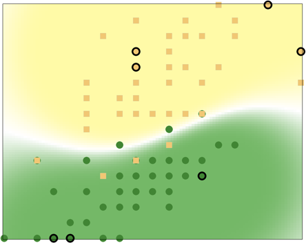
prtClassNnet enables automatic visualization of the algorithm progress as learning proceeds. You can set how often (or whether) this visualization occurs by setting nnet.plotOnIter to a scalar; the scalar represents how often to update the plots. Use 0 to use no visualization.
Example Processing
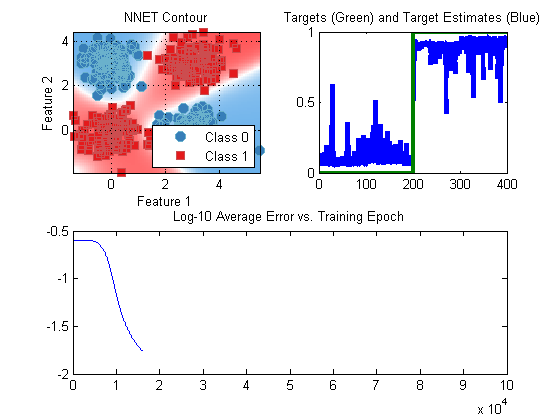
So, what does the resulting process look like? Let’s give it a whirl with a stadnard X-OR data set:
dsTrain = prtDataGenXor;
dsTest = prtDataGenXor;
nnet = prtClassNnet('nHiddenUnits',10,'plotOnIter',1000,'relativeErrorChangeThreshold',1e-4);
nnet = nnet.train(dsTrain);
yOut = nnet.run(dsTest);
Concluding
We hope that using prtClassNnet enables you to do some new, neat things. If you like it, please help us re-write the code to overcome our current restrictions!
Happy coding.