Hi everyone, today I wanted to introduce a new data set and some preliminary processing that helps us perform better than a random forest (gasp!).
The data we’re going to use is from a Kaggle competition that’s going on from now (March 28, 2013) until April 15, 2013. Kaggle is a company that specializes in connecting data analysts with interesting data - it’s pretty great for hobbyists and individuals to get started with some data, and potentially win some money! And they just generally have a lot of cool data from a lot of interesting problems.
The data we’re going to use is based on identifying an author’s gender from samples of their handwriting. Here’s the URL for the competition home page, which gives some details on the data:
http://www.kaggle.com/c/icdar2013-gender-prediction-from-handwriting
The competition includes several sets of images,as well as some pre-extracted features. The image files can be gigantic, so we’re only going to use the pre-extracted features for today. Go ahead and download train.csv, train_answers.csv, and test.csv, from the link above, and put them in
fullfile(prtRoot,'dataGen','dataStorage','kaggleTextGender_2013');
Once the files are in the correct location, you should be able to use:
[dsTrain,dsTest] = prtDataGenTextGender;
to load in the data.
Contents
M-Files You Need
Obviously, prtDataGenTextGender.m is new, as are a number of other files we’re going to use throughout this example. These include prtEvalLogLoss.m, prtScoreLogLoss.m, prtUtilAccumArrayLike.m, and prtUtilAccumDataSetLike.m. You’ll need to update your PRT to the newest version (as of March, 2013, anyway) to get access to these files. You can always get the PRT here: http://github.com/newfolder/PRT
Once you’ve done all that, go ahead and try the following:
[dsTrain,dsTest] = prtDataGenTextGender;
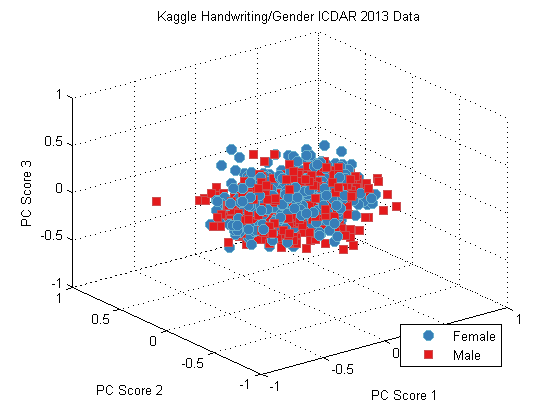
That should load in the data. As always, we can visualize the data using someting simple, like PCA:
pca = prtPreProcPca;
pca = pca.train(dsTrain);
dsPca = pca.run(dsTrain);
plot(dsPca);
title('Kaggle Handwriting/Gender ICDAR 2013 Data');
Naive Random Forest
Kaggle competitions will often provide a baseline performance metric for some standard classification algorithms. In this example they told us that the baseline random forest performamce they’ve observed obtains a log-loss of about 0.65. We can confirm this using our random forest, 3-fold cross-validation, and our new function prtScoreLogLoss:
yOut = kfolds(prtClassTreeBaggingCap,dsTrain,3);
logLossInitialRf = prtScoreLogLoss(yOut);
fprintf(‘Random Forest LogLoss: %.2f\n’,logLossInitialRf);
Random Forest LogLoss: 0.64
About 0.65, so we’re right in the ball-park. Can we do better?
Remove Meaningless features
That performance wasn’t that great. And the leaderboard shows us that some clever people have already done significantly better than the basic random forest.
Let’s investigate the data a little and see what’s going on. First, what is the standard deviation of the features?
stem(log(std(dsTrain.X)));
xlabel(‘Feature Number’);
ylabel(‘Log-\sigma’);
title(‘Log(\sigma) vs. Feature Number’);
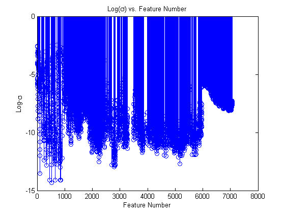
Wow, there are a lot of features with a standard deviation of zero! That means that we can’t learn anything from these features, since they always take the exact same value in the training set. Let’s go ahead and remove these features.
fprintf(‘There are %d features that only take one value… \n’,length(find(std(dsTrain.X)==0)));
removeFeats = std(dsTrain.X) == 0;
dsTrainRemove = dsTrain.removeFeatures(removeFeats);
dsTestRemove = dsTest.removeFeatures(removeFeats);
There are 2414 features that only take one value…
Slight improvement
What happens if we re-run the random forest on this data with the new features removed? The random forest is pretty robust to meaningless features, but not totally impervious… let’s try it:
yOutRf = kfolds(prtClassTreeBaggingCap,dsTrainRemove,3);
logLossRfFeatsRemoved = prtScoreLogLoss(yOutRf);
fprintf(‘Random Forest LogLoss with meaningless features removed: %.2f\n’,logLossRfFeatsRemoved);
Random Forest LogLoss with meaningless features removed: 0.61
Hey! That did marginally better – our log-loss went from about 0.65 to 0.61 or so. Nothing to write home about, but a slight improvement. What else can we do?
Aggregating Over Writers
If you pay attention to the data set, you’ll notice something interesting – we have a lot of writing samples (4) from each writer. And our real goal is to identify the gender of each writer – so we should be able to average our classifications over each writer and get better performance.
This blog entry introduces a new function called “prtUtilAccumDataSetLike”, which acts a lot like “accumarray” in base MATLAB. Basically, prtUtilAccumDataSetLike takes a set of keys of size dataSet.nObservations x 1, and for each observation corresponding to each unique key, aggregates the data in X and Y and outputs a new data set.
It’s a little complicated to explain – take a look at the help entry for accumarray, and then take a look at this example:
writerIds = [dsTrainRemove.observationInfo.writerId]‘;
yOutAccum = prtUtilAccumDataSetLike(writerIds,yOutRf,@(x)mean(x));
The code above outputs a new data set generated by averaging the confidences in yOutRf across sets of writerIds.
Does this help performance?
logLossAccum = prtScoreLogLoss(yOutAccum);
fprintf('Writer ID Accumulated Random Forest LogLoss: %.2f\n’,logLossAccum);
Writer ID Accumulated Random Forest LogLoss: 0.59
That’s marginally better still! What else can we try…
PLSDA
When a random forest seems to be doing somewhat poorly, often it’s a good idea to take a step back and run a linear classifier in lieu of a nice fancy random forest. I’m partial to PLSDA as a classifier (see the help entry for prtClassPlsda for more information).
PLSDA has one parameter – the number of components to use, that we should optimize over. Since each kfolds-run is random, we’ll run 10 experiments of 3-Fold Cross-validation for each of 1 – 30 components in PLSDA… This might take a little while depending on your computer…
We’re also going to do something a little tricky here – PLSDA is a linear classifier, and won’t output values between zero and one by default. But the outputs from PLSDA should be linearly correlated with confidence that the author of a particular text was a male. We can translate from PLSDA outputs to values with probabilistic interpretations by attaching a logistic-discriminant function to the end of our PLSDA classifier. That’s easy to do in the PRT like so:
classifier = prtClassPlsda(‘nComponents’,nComp) + prtClassLogisticDiscriminant;
nIter = 10; maxComp = 30; logLossPlsda = nan(maxComp,nIter); logLossPlsdaAccum = nan(maxComp,nIter); for nComp = 1:maxComp;classifier = prtClassPlsda(<span class="string">'nComponents'</span>,nComp) + prtClassLogisticDiscriminant; classifier.showProgressBar = false; <span class="keyword">for</span> iter = 1:nIter yOutPlsda = kfolds(classifier,dsTrainRemove,3); logLossPlsda(nComp,iter) = prtScoreLogLoss(yOutPlsda); yOutAccum = prtUtilAccumDataSetLike(writerIds,yOutPlsda,@(x)mean(x)); logLossPlsdaAccum(nComp,iter) = prtScoreLogLoss(yOutAccum); <span class="keyword">end</span> fprintf(<span class="string">'%d '</span>,nComp);end fprintf(‘\n’);
1 2 3 4 5 6 7 8 9 10 11 12 13 14 15 16 17 18 19 20 21 22 23 24 25 26 27 28 29 30
Plotting Results
Let’s take a look at the PLSDA classifier performance as a function of the number of components we used. The following code generates box-plots (recall, we ran 3-fold cross-validation 10 times for each # of components between 1 and 30…
boxplot(logLossPlsdaAccum')
hold on;
h2 = plot(1:maxComp,repmat(logLossInitialRf,1,maxComp),‘k:’,1:maxComp,repmat(logLossRfFeatsRemoved,1,maxComp),‘b:’,1:maxComp,repmat(logLossAccum,1,maxComp),‘g:’);
hold off;
legend(h2,{‘Random Forest Log-Loss’,‘Random Forest – Removed Features’,‘Random Forest – Removed Features – Accum’});
h = findobj(gca,‘type’,‘line’);
set(h,‘linewidth’,2);
xlabel(‘#PLSDA Components’);
ylabel(‘Log-Loss’);
title(‘Log-Loss For PLSDA With Accumumation (vs. # Components) and Random Forest’)
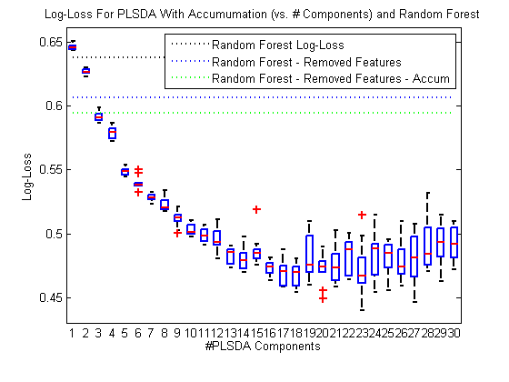
Wow! The dotted lines here represent the random forest performance we’ve seen, and the boxes represent the performance we get with PLSDA – PLSDA is significantly outperforming our RF classifier on this data!
PLSDA performance seems to plateau around 17 components, so we’ll use 17 from now on.
Submit it!
I think we might have something here – our code gets Log-Losses around 0.46 many times. Let’s actually submit an experiment to Kaggle.
First we’ll train our classifier and test it:
classifier = prtClassPlsda(‘nComponents’,17) + prtClassLogisticDiscriminant; classifier = classifier.train(dsTrainRemove); yOutTest = classifier.run(dsTestRemove);writerIdsTest = [dsTestRemove.observationInfo.writerId]‘;
Don’t forget to accumulate:
[yOutPlsdaTestAccum,uKeys] = prtUtilAccumDataSetLike(writerIdsTest,yOutTest,@(x)mean(x));
matrixOut = cat(2,uKeys,yOutPlsdaTestAccum.X);
And write the output the way Kaggle wants us to.
csvwrite('outputPlsda.csv’,matrixOut);
Results
I made a screen-cap of the results from the output above – here it is:
imshow(‘leaderBoard_2013_03_20.PNG’);
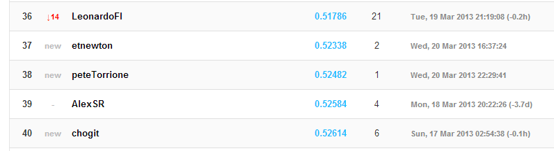
That’s me in the middle there – #38 out of about 100. And way better than the naive random forest implementation – not too bad!
Can we do better?
Feature Selection
One way we can reduce variation and improve performance is to not include all 4652 features left in our data set. We can use feature selection to pick the ones we want!
I’m going to go ahead and warn you – don’t run this code unless you want to leave it running overnight. It takes forever… but it gets the job done:
warning off;
c = prtClassPlsda('nComponents' ,17, 'showProgressBar',false);
sfs = prtFeatSelSfs('nFeatures',100, 'evaluationMetric',@(ds)-1*prtEvalLogLoss(c,ds,2));
sfs = sfs.train(dsTrainRemove);
Instead, we already ran that code, and saved the results in sfs.mat, which you can down-load at the end of this post.
For now, let’s look at how performance is affected by the number of features retained:
load sfs.mat sfs
set(gcf,'position',[403   246   560   420]); %fix from IMSHOW
plot(-sfs.performance)
xlabel('# Features');
ylabel('Log-Loss');
title('Log-Loss vs. # Features Retained');
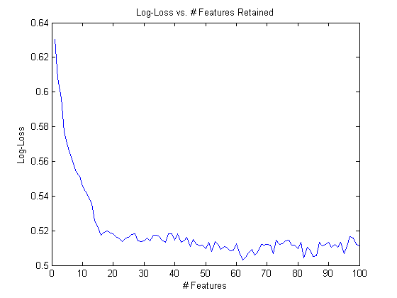
It looks like performance is bottoming out around 60 or so features, and anything past that isn’t adding performance (though maybe if we selected 1000 or 2000 we could do better!)
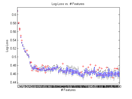
We can confirm this with the following code, which also takes quite a while to run a bunch of experiments on all the sub-sets SFS found for us:
logLossClassifierFeatSel = nan(100,10); for nFeats = 1:100;<span class="keyword">for</span> iter = 1:10 dsTrainRemoveFeatSel = dsTrainRemove.retainFeatures(sfs.selectedFeatures(1:nFeats)); yOutPlsdaFeatSel = classifier.kfolds(dsTrainRemoveFeatSel,3); xOutAccum = prtUtilAccumArrayLike(writerIds,yOutPlsdaFeatSel.X,[],@(x)mean(x)); yOutAccum = prtUtilAccumArrayLike(writerIds,yOutPlsdaFeatSel.Y,[],@(x)unique(x)); yOutAccumFeatSel = prtDataSetClass(xOutAccum,yOutAccum); logLossClassifierFeatSel(nFeats,iter) = prtScoreLogLoss(yOutAccumFeatSel); <span class="keyword">end</span>end
boxplot(logLossClassifierFeatSel’) drawnow;
ylabel(‘Log-Loss’); xlabel(‘# Features’) title(‘Log-Loss vs. # Features’)
Adding in some post-processing
In a minute we’ll down-select the number of features we want to use – but first let’s do one more thing. Recall that we added a logistic discriminant at the end of our PLSDA classifier. That was clever, but after that, we accumulted a bunch of data together. We might be able to run another logistic discriminant after the accumultion to do even better!
Let’s see what that code looks like:
classifier = prtClassPlsda(‘nComponents’,17) + prtClassLogisticDiscriminant; classifier = classifier.train(dsTrainRemove); yOutPlsdaKfolds = classifier.kfolds(dsTrainRemove,3);yOutAccum = prtUtilAccumDataSetLike(writerIds,yOutPlsdaKfolds,@(x)mean(x)); yOutAccumLogDisc = kfolds(prtClassLogisticDiscriminant,yOutAccum,3);
logLossPlsdaAccum = prtScoreLogLoss(yOutAccum); logLossPlsdaAccumLogDisc = prtScoreLogLoss(yOutAccumLogDisc); fprintf(‘Without post-Log-Disc: %.3f; With: %.3f\n’,logLossPlsdaAccum,logLossPlsdaAccumLogDisc);
Without post-Log-Disc: 0.479; With: 0.461
That’s a slight improvement, too!
Our New Submission
Let’s put everything together, and see what happens:
First, pick the right # of features based on our big experiment above:
[minVal,nFeatures] = min(mean(logLossClassifierFeatSel'));
dsTrainTemp = dsTrainRemove.retainFeatures(sfs.selectedFeatures(1:nFeatures));
dsTestTemp = dsTestRemove.retainFeatures(sfs.selectedFeatures(1:nFeatures));
Now, train a classifier, and a logistic discriminant:
classifier = prtClassPlsda(‘nComponents’,17) + prtClassLogisticDiscriminant; classifier = classifier.train(dsTrainRemove); yOutPlsdaKfolds = classifier.kfolds(dsTrainRemove,3);yOutAccum = prtUtilAccumDataSetLike(writerIds,yOutPlsdaKfolds,@(x)mean(x)); yOutPostLogDisc = kfolds(prtClassLogisticDiscriminant,yOutAccum,3); postLogDisc = train(prtClassLogisticDiscriminant,yOutAccum); logLossPlsdaEstimate = prtScoreLogLoss(yOutPostLogDisc);
And run the same classifier, followed by the post-processing logistic discriminant:
yOut = classifier.run(dsTestRemove); [xOutAccumSplit,uLike] = prtUtilAccumDataSetLike(writerIdsTest,yOut,@(x)mean(x)); dsTestPost = prtDataSetClass(xOutAccumSplit); yOutPost = postLogDisc.run(dsTestPost);matrixOut = cat(2,uLike,yOutPost.X); csvwrite(‘outputPlsda_FeatSelPostProc.csv’,matrixOut);
Final Results
We submitted this version to Kaggle also. The results are shown below:
imshow(‘leaderBoard_2013_03_21.PNG’);
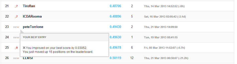
That bumped us up by just a little bit in terms of overall log-loss, but quite a bit in the leader-list!
A lot of people are still doing way better than this blog entry (and have gotten better since a week ago, when we did this analysis!), but that’s not bad performance for what turns out to be about 20 lines of code, don’t you think?
If you have any success with the text/gender analysis data using the PRT, let us know – either post on the Kaggle boards, or here, or drop us an e-mail.